
face_beautification.markdown 18 KB
Implementing a face beautification algorithm with G-API {#tutorial_gapi_face_beautification}
@prev_tutorial{tutorial_gapi_anisotropic_segmentation}
[TOC]
Introduction {#gapi_fb_intro}
In this tutorial you will learn:
- Basics of a sample face beautification algorithm;
- How to infer different networks inside a pipeline with G-API;
- How to run a G-API pipeline on a video stream.
Prerequisites {#gapi_fb_prerec}
This sample requires:
- PC with GNU/Linux or Microsoft Windows (Apple macOS is supported but was not tested);
- OpenCV 4.2 or later built with Intel® Distribution of OpenVINO™ Toolkit (building with Intel® TBB is a plus);
- The following topologies from OpenVINO™ Toolkit Open Model
Zoo:
face-detection-adas-0001;facial-landmarks-35-adas-0002.
Face beautification algorithm {#gapi_fb_algorithm}
We will implement a simple face beautification algorithm using a combination of modern Deep Learning techniques and traditional Computer Vision. The general idea behind the algorithm is to make face skin smoother while preserving face features like eyes or a mouth contrast. The algorithm identifies parts of the face using a DNN inference, applies different filters to the parts found, and then combines it into the final result using basic image arithmetics:
\dot strict digraph Pipeline { node [shape=record fontname=Helvetica fontsize=10 style=filled color="#4c7aa4" fillcolor="#5b9bd5" fontcolor="white"]; edge [color="#62a8e7"]; ordering="out"; splines=ortho; rankdir=LR;
input [label="Input"]; fd [label="Face\ndetector"]; bgMask [label="Generate\nBG mask"]; unshMask [label="Unsharp\nmask"]; bilFil [label="Bilateral\nfilter"]; shMask [label="Generate\nsharp mask"]; blMask [label="Generate\nblur mask"]; mul_1 [label="" fontsize=24 shape=circle labelloc=b]; mul_2 [label="" fontsize=24 shape=circle labelloc=b]; mul_3 [label="*" fontsize=24 shape=circle labelloc=b];
subgraph cluster_0 {
style=dashed
fontsize=10
ld [label="Landmarks\ndetector"];
label="for each face"
}
sum_1 [label="+" fontsize=24 shape=circle]; out [label="Output"];
temp_1 [style=invis shape=point width=0]; temp_2 [style=invis shape=point width=0]; temp_3 [style=invis shape=point width=0]; temp_4 [style=invis shape=point width=0]; temp_5 [style=invis shape=point width=0]; temp_6 [style=invis shape=point width=0]; temp_7 [style=invis shape=point width=0]; temp_8 [style=invis shape=point width=0]; temp_9 [style=invis shape=point width=0];
input -> temp_1 [arrowhead=none] temp_1 -> fd -> ld ld -> temp_4 [arrowhead=none] temp_4 -> bgMask bgMask -> mul_1 -> sum_1 -> out
temp_4 -> temp_5 -> temp_6 [arrowhead=none constraint=none] ld -> temp_2 -> temp_3 [style=invis constraint=none]
temp_1 -> {unshMask, bilFil} fd -> unshMask [style=invis constraint=none] unshMask -> bilFil [style=invis constraint=none]
bgMask -> shMask [style=invis constraint=none] shMask -> blMask [style=invis constraint=none] mul_1 -> mul_2 [style=invis constraint=none] temp_5 -> shMask -> mul_2 temp_6 -> blMask -> mul_3
unshMask -> temp_2 -> temp_5 [style=invis] bilFil -> temp_3 -> temp_6 [style=invis]
mul_2 -> temp_7 [arrowhead=none] mul_3 -> temp_8 [arrowhead=none]
temp_8 -> temp_7 [arrowhead=none constraint=none] temp_7 -> sum_1 [constraint=none]
unshMask -> mul_2 [constraint=none] bilFil -> mul_3 [constraint=none] temp_1 -> mul_1 [constraint=none] } \enddot
Briefly the algorithm is described as follows:
- Input image \f$I\f$ is passed to unsharp mask and bilateral filters (\f$U\f$ and \f$L\f$ respectively);
- Input image \f$I\f$ is passed to an SSD-based face detector;
- SSD result (a \f$[1 \times 1 \times 200 \times 7]\f$ blob) is parsed and converted to an array of faces;
- Every face is passed to a landmarks detector;
- Based on landmarks found for every face, three image masks are
generated:
- A background mask \f$b\f$ -- indicating which areas from the original image to keep as-is;
- A face part mask \f$p\f$ -- identifying regions to preserve (sharpen).
- A face skin mask \f$s\f$ -- identifying regions to blur;
- The final result \f$O\f$ is a composition of features above calculated as \f$O = b*I + p*U + s*L\f$.
Generating face element masks based on a limited set of features (just 35 per face, including all its parts) is not very trivial and is described in the sections below.
Constructing a G-API pipeline {#gapi_fb_pipeline}
Declaring Deep Learning topologies {#gapi_fb_decl_nets}
This sample is using two DNN detectors. Every network takes one input and produces one output. In G-API, networks are defined with macro G_API_NET():
@snippet cpp/tutorial_code/gapi/face_beautification/face_beautification.cpp net_decl
To get more information, see Declaring Deep Learning topologies described in the "Face Analytics pipeline" tutorial.
Describing the processing graph {#gapi_fb_ppline}
The code below generates a graph for the algorithm above:
@snippet cpp/tutorial_code/gapi/face_beautification/face_beautification.cpp ppl
The resulting graph is a mixture of G-API's standard operations,
user-defined operations (namespace custom::), and DNN inference.
The generic function cv::gapi::infer<>() allows to trigger inference
within the pipeline; networks to infer are specified as template
parameters. The sample code is using two versions of cv::gapi::infer<>():
- A frame-oriented one is used to detect faces on the input frame.
- An ROI-list oriented one is used to run landmarks inference on a list of faces -- this version produces an array of landmarks per every face.
More on this in "Face Analytics pipeline" (Building a GComputation section).
Unsharp mask in G-API {#gapi_fb_unsh}
The unsharp mask \f$U\f$ for image \f$I\f$ is defined as:
\f[U = I - s * L(M(I)),\f]
where \f$M()\f$ is a median filter, \f$L()\f$ is the Laplace operator, and \f$s\f$ is a strength coefficient. While G-API doesn't provide this function out-of-the-box, it is expressed naturally with the existing G-API operations:
@snippet cpp/tutorial_code/gapi/face_beautification/face_beautification.cpp unsh
Note that the code snipped above is a regular C++ function defined with G-API types. Users can write functions like this to simplify graph construction; when called, this function just puts the relevant nodes to the pipeline it is used in.
Custom operations {#gapi_fb_proc}
The face beautification graph is using custom operations extensively. This chapter focuses on the most interesting kernels, refer to G-API Kernel API for general information on defining operations and implementing kernels in G-API.
Face detector post-processing {#gapi_fb_face_detect}
A face detector output is converted to an array of faces with the following kernel:
@snippet cpp/tutorial_code/gapi/face_beautification/face_beautification.cpp vec_ROI @snippet cpp/tutorial_code/gapi/face_beautification/face_beautification.cpp fd_pp
Facial landmarks post-processing {#gapi_fb_landm_detect}
The algorithm infers locations of face elements (like the eyes, the mouth and the head contour itself) using a generic facial landmarks detector (details) from OpenVINO™ Open Model Zoo. However, the detected landmarks as-is are not enough to generate masks --- this operation requires regions of interest on the face represented by closed contours, so some interpolation is applied to get them. This landmarks processing and interpolation is performed by the following kernel:
@snippet cpp/tutorial_code/gapi/face_beautification/face_beautification.cpp ld_pp_cnts
The kernel takes two arrays of denormalized landmarks coordinates and returns an array of elements' closed contours and an array of faces' closed contours; in other words, outputs are, the first, an array of contours of image areas to be sharpened and, the second, another one to be smoothed.
Here and below Contour is a vector of points.
Getting an eye contour {#gapi_fb_ld_eye}
Eye contours are estimated with the following function:
@snippet cpp/tutorial_code/gapi/face_beautification/face_beautification.cpp ld_pp_incl @snippet cpp/tutorial_code/gapi/face_beautification/face_beautification.cpp ld_pp_eye
Briefly, this function restores the bottom side of an eye by a
half-ellipse based on two points in left and right eye
corners. In fact, cv::ellipse2Poly() is used to approximate the eye region, and
the function only defines ellipse parameters based on just two points:
- The ellipse center and the \f$X\f$ half-axis calculated by two eye Points;
- The \f$Y\f$ half-axis calculated according to the assumption that an average eye width is \f$1/3\f$ of its length;
- The start and the end angles which are 0 and 180 (refer to
cv::ellipse()documentation); - The angle delta: how much points to produce in the contour;
- The inclination angle of the axes.
The use of the atan2() instead of just atan() in function
custom::getLineInclinationAngleDegrees() is essential as it allows to
return a negative value depending on the x and the y signs so we
can get the right angle even in case of upside-down face arrangement
(if we put the points in the right order, of course).
Getting a forehead contour {#gapi_fb_ld_fhd}
The function approximates the forehead contour:
@snippet cpp/tutorial_code/gapi/face_beautification/face_beautification.cpp ld_pp_fhd
As we have only jaw points in our detected landmarks, we have to get a half-ellipse based on three points of a jaw: the leftmost, the rightmost and the lowest one. The jaw width is assumed to be equal to the forehead width and the latter is calculated using the left and the right points. Speaking of the \f$Y\f$ axis, we have no points to get it directly, and instead assume that the forehead height is about \f$2/3\f$ of the jaw height, which can be figured out from the face center (the middle between the left and right points) and the lowest jaw point.
Drawing masks {#gapi_fb_masks_drw}
When we have all the contours needed, we are able to draw masks:
@snippet cpp/tutorial_code/gapi/face_beautification/face_beautification.cpp msk_ppline
The steps to get the masks are:
- the "sharp" mask calculation:
- fill the contours that should be sharpened;
- blur that to get the "sharp" mask (
mskSharpG);
- the "bilateral" mask calculation:
- fill all the face contours fully;
- blur that;
- subtract areas which intersect with the "sharp" mask --- and get the
"bilateral" mask (
mskBlurFinal);
- the background mask calculation:
- add two previous masks
- set all non-zero pixels of the result as 255 (by
cv::gapi::threshold()) - revert the output (by
cv::gapi::bitwise_not) to get the background mask (mskNoFaces).
Configuring and running the pipeline {#gapi_fb_comp_args}
Once the graph is fully expressed, we can finally compile it and run on real data. G-API graph compilation is the stage where the G-API framework actually understands which kernels and networks to use. This configuration happens via G-API compilation arguments.
DNN parameters {#gapi_fb_comp_args_net}
This sample is using OpenVINO™ Toolkit Inference Engine backend for DL inference, which is configured the following way:
@snippet cpp/tutorial_code/gapi/face_beautification/face_beautification.cpp net_param
Every cv::gapi::ie::Params<> object is related to the network
specified in its template argument. We should pass there the network
type we have defined in G_API_NET() in the early beginning of the
tutorial.
Network parameters are then wrapped in cv::gapi::NetworkPackage:
@snippet cpp/tutorial_code/gapi/face_beautification/face_beautification.cpp netw
More details in "Face Analytics Pipeline" (Configuring the pipeline section).
Kernel packages {#gapi_fb_comp_args_kernels}
In this example we use a lot of custom kernels, in addition to that we use Fluid backend to optimize out memory for G-API's standard kernels where applicable. The resulting kernel package is formed like this:
@snippet cpp/tutorial_code/gapi/face_beautification/face_beautification.cpp kern_pass_1
Compiling the streaming pipeline {#gapi_fb_compiling}
G-API optimizes execution for video streams when compiled in the "Streaming" mode.
@snippet cpp/tutorial_code/gapi/face_beautification/face_beautification.cpp str_comp
More on this in "Face Analytics Pipeline" (Configuring the pipeline section).
Running the streaming pipeline {#gapi_fb_running}
In order to run the G-API streaming pipeline, all we need is to
specify the input video source, call
cv::GStreamingCompiled::start(), and then fetch the pipeline
processing results:
@snippet cpp/tutorial_code/gapi/face_beautification/face_beautification.cpp str_src @snippet cpp/tutorial_code/gapi/face_beautification/face_beautification.cpp str_loop
Once results are ready and can be pulled from the pipeline we display it on the screen and handle GUI events.
See Running the pipeline section in the "Face Analytics Pipeline" tutorial for more details.
Conclusion {#gapi_fb_cncl}
The tutorial has two goals: to show the use of brand new features of G-API introduced in OpenCV 4.2, and give a basic understanding on a sample face beautification algorithm.
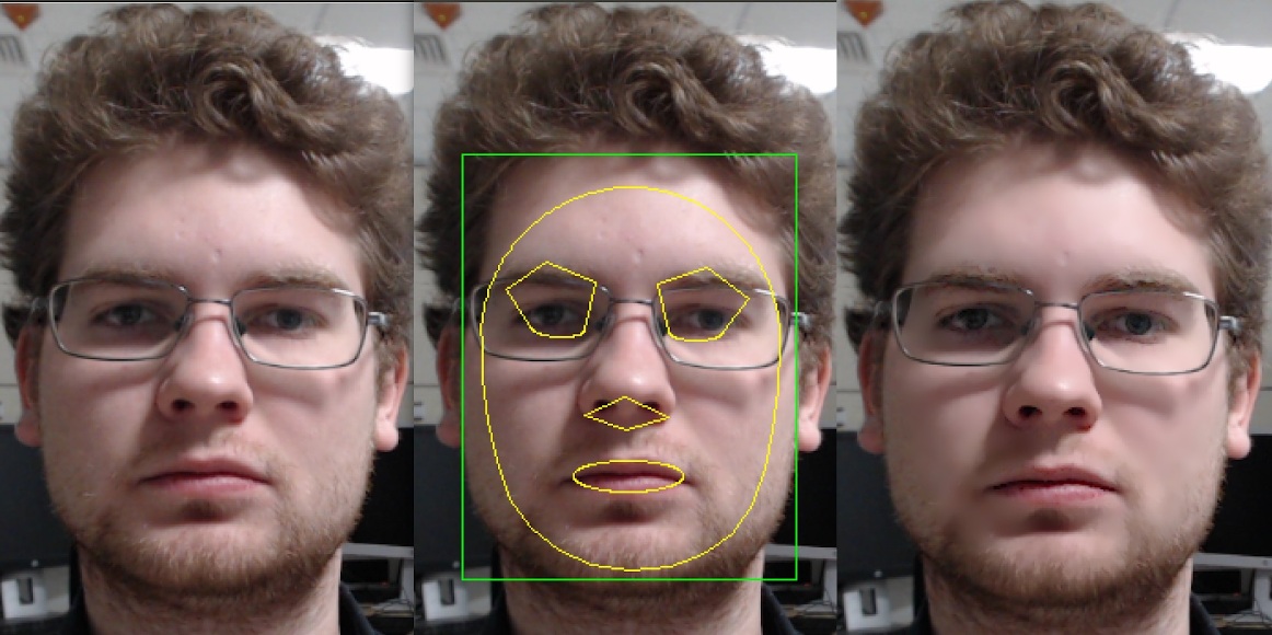
The result of the algorithm application:
On the test machine (Intel® Core™ i7-8700) the G-API-optimized video pipeline outperforms its serial (non-pipelined) version by a factor of 2.7 -- meaning that for such a non-trivial graph, the proper pipelining can bring almost 3x increase in performance.